Thermodynamic & fluid-system modeling

State the physics you know. Solve for everything else.

Draw a connected system. Specify the conditions you actually know. The solver finds every remaining pressure, temperature, phase, and mass flow — coupled, not copy-pasted between calculations.

EARLY ACCESS · v0.5.0 · SOLVER UNDER ACTIVE VALIDATION
CONDENSER EVAPORATOR COMP TXV suction line · DN22 discharge line liquid line + bend Q̇ = 9.07 kW Q̇ = 6.76 kW Ẇ = 2.31 kW 1 186 kPa ΔT_sh 8.0 K 3 1.02 MPa 68.1 °C 5 1.00 MPa ΔT_sc 5.0 K 7 214 kPa x = 0.289
↓ SCROLL — THE SYSTEM BELOW IS SOLVED STEP BY STEP
137 working fluids 19 component models F(x) = 0 over real equations of state 100% local computation

The product

An engineering workspace, not a stack of calculators.

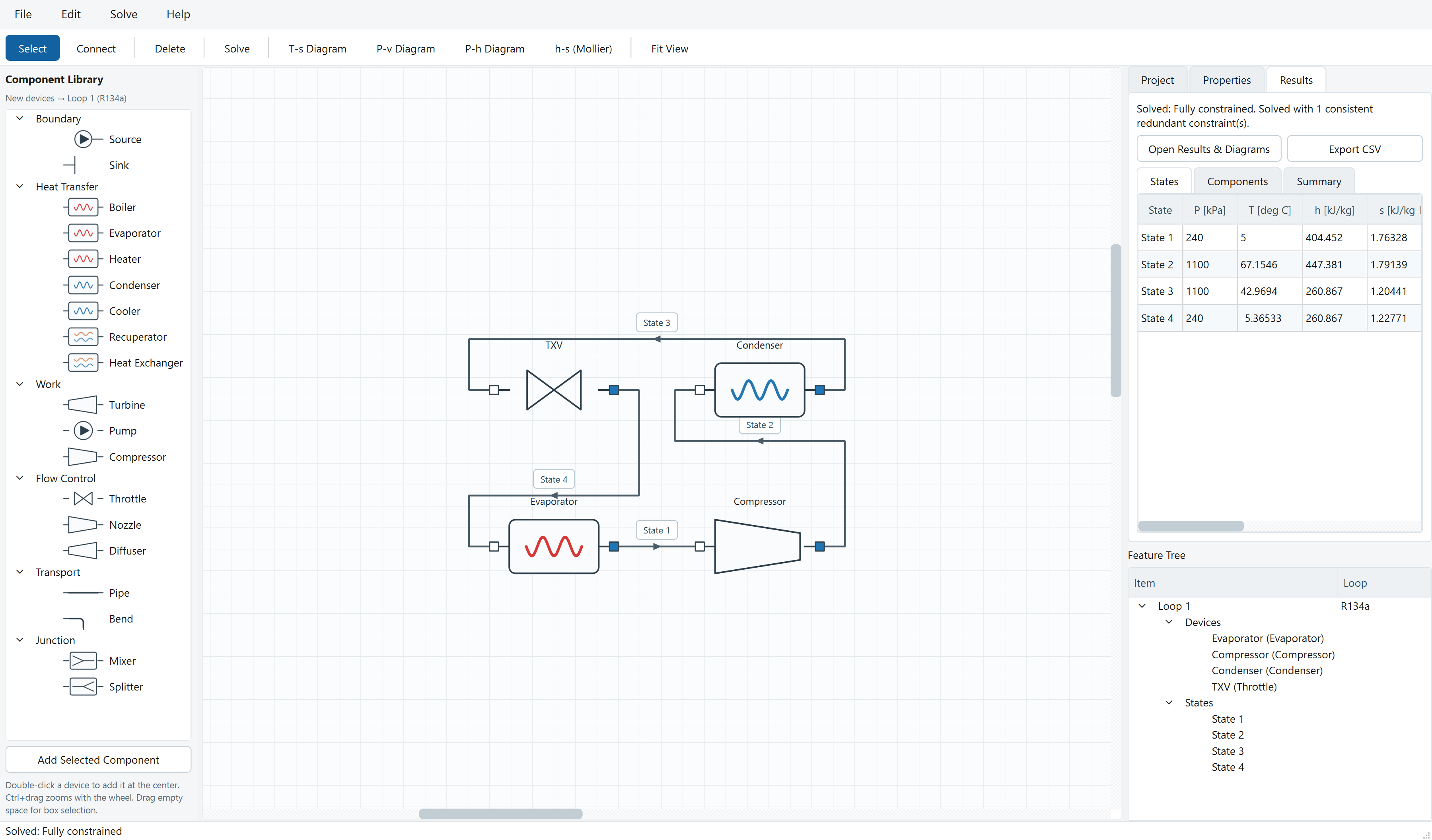
Schematic canvas, docked project and properties panels, live state labels, property diagrams, CSV export. This is the actual application.

The ThermoFluid Studio application: a refrigeration cycle drawn on the schematic canvas with the component library, properties panel, and results tabs visible
Library — drag components onto the canvas
Loops — independent fluids per loop
Results — states, components, diagrams
Canvas — routed connections, live state labels

Why coupled

From scattered calculations to one model.

Spreadsheets, property tables, and scripts are fine tools. The difference is the coupling: change one condition here and every downstream state updates in the same solve.

The usual way
property tables — look up h, s by hand
spreadsheet — energy balances, cell by cell
separate ΔP calculation — friction, bends
re-enter results upstream — and hope nothing drifted
repeat until it stops changing
ThermoFluid Studio
build the connected system
specify the conditions you know
solve the coupled model
inspect every state, residual, and diagram

One representation. The pressure drop, the compressor work, and the phase at every point come out of the same F(x) = 0.

01 — CONSTRAIN

You don't fill in forms. You state what you know.

Pin the pressures you know. Demand superheat and subcooling. The environment counts degrees of freedom until the system is exactly solvable.

unknowns (P, h × 7 states)14
component residuals0 / 8
specifications0 / 6
degrees of freedom14
statusunderconstrained
CONDENSER EVAPORATOR COMP suction line discharge line liquid line P₁ = 186 kPa (suction) ΔT_sh = 8.0 K η_s = 0.72 P₅ = 1.00 MPa (cond) ΔT_sc = 5.0 K ṁ = 0.045 kg/s

02 — SOLVE

One coupled system. Nothing linearized behind your back.

Friction correlations, efficiency relations, phase conditions — every component contributes its residuals to F(x) = 0, solved whole. Rank analysis proves your specifications actually determine the answer.

systemF: ℝ¹⁴ → ℝ¹⁴
jacobian14×14 · nnz 56 · FD
rank(J) — SVD14 / 14
methodtrust-region reflective
statusiterating…
r₀₃suction line P₁ − P₂ − f·(L/D)·½ρV̄² = 0,  f = 0.25 / [log₁₀(ε/3.7D + 5.74/Re⁰·⁹)]² → 1.8e−12
r₀₅compressor h₃ − h₂ − [h(P₃, s(P₂,h₂)) − h₂] / η_s = 0 → 4.1e−12
r₀₈condenser outlet T₅(P₅,h₅) − T_sat(P₅) + ΔT_sc = 0 → 2.6e−11
r₁₁expansion valve h₇ − h₆ = 0  (isenthalpic) → 0.0
r₁₃evaporator ṁ(h₁ − h₇) − Q̇_ev = 0,  T₁ − T_sat(P₁) − ΔT_sh = 0 → 3.2e−11
jacobian sparsity · 14×14
Each row is one equation, each column one unknown. Filled cells: which equations touch which unknowns.
trust-region iterations
it‖F‖∞‖Δx‖
04.2e+02
16.8e+012.1e−01
23.4e+008.7e−02
31.2e−011.1e−02
48.6e−046.3e−04
52.4e−062.9e−05
68.1e−091.4e−06
73.2e−115.0e−08
The worst residual falls thirteen orders of magnitude — then the solver stops and reports it, rather than rounding it away.

03 — VERIFY

A result you can check, not just accept.

The dome is computed from the equation of state, the cycle sits where the physics puts it — superheat and subcooling visibly outside the dome — and the first law must close. Every time.

Q̇_evap + Ẇ_comp6.76 + 2.31 kW
Q̇_cond + lines9.07 kW
first-law closure0.42 kW
COP
And when a specification set is wrong, it says so. Impose x₇ = 0.10 against these pressures and the report reads overconstrained / inconsistent — naming the offending residual — instead of averaging the conflict away.
specific enthalpy h [kJ/kg] pressure P [kPa, log]

04 — INTERACT

Move the physics yourself.

Three specifications a real system lives or dies by. Watch flash quality, discharge temperature, and COP respond.

PREPARED DEMONSTRATION · 250 PRECOMPUTED SOLUTIONS specific enthalpy h [kJ/kg] pressure P [kPa, log]
1000 kPa
8 K
5 K
pressure ratio P₃/P₂5.49
T₃ — discharge temperature68.1 °C
x₇ — flash quality after valve0.289
Q̇_evap — cooling capacity6.76 kW
Ẇ_comp — compressor power2.31 kW
Q̇_rej — total heat rejected9.07 kW
COP — coefficient of performance2.92

R134a · suction 186 kPa after coil + line drop from a 214 kPa evaporator inlet · discharge at P_cond + 22 kPa · η_s = 0.72 · ṁ = 0.045 kg/s. In the application these are live solves over any of 137 fluids; here they are precomputed because this page ships no solver.

Applications

One solver. Any loop.

The same constraint formulation, from refrigeration plants to microreactors.

BUNDLED EXAMPLE COND EVAP COP 2.92 · x₇ 0.29 · ΔT_sh 8 K

Refrigeration & heat pumps

Vapor-compression with superheat, subcooling, and line losses.

R134a · CO₂ · NH₃ · propane
BUNDLED EXAMPLE BLR TRB CND P η_th · x_exhaust

Steam power

Rankine cycles, boiler to condensate return, with recuperation.

Water/steam · 8 MPa · turbine η_s
BUNDLED EXAMPLE CORE T C RCP He · closed loop

Closed-loop gas power

Recuperated Brayton, down to microreactor scale.

Helium · CO₂ · back-work ratio
COMPONENTS AVAILABLE Δz 40 m f(Re, ε/D)

Pumped liquid networks

Static head, long runs, bends — friction and pump work together.

Darcy–Weisbach · Crane K · DN80
COMPONENTS AVAILABLE C RCP N₂ · 77 K

Cryogenics

JT throttling and recuperative cooling toward liquefaction.

N₂ · H₂ · methane · throttle h=const
COMPONENTS AVAILABLE HTR T CND P kW_th → kW_e

Waste-heat recovery

Organic Rankine loops from low-grade heat.

R245fa · n-Pentane · toluene

BUNDLED EXAMPLE — ships as a working sample project you can open and solve. COMPONENTS AVAILABLE — the required components and fluids ship today; you build the model yourself. Neither label is a certification for any particular engineering use.

Trust

Built to show its work.

Every result carries its derivation. Nothing is a number without a pedigree.

  • governing equations, per component
  • assumptions and model limits
  • every specification you imposed
  • degrees of freedom and rank
  • property model per fluid
  • solver status and iterations
  • residual at every equation
  • energy-balance closure
  • units on every quantity
  • intermediate state values
CaseChecked againstLayerStatus
R134a vapor-compression cyclefirst-law closure, COPintegrationPASSING IN CI
Helium closed Brayton (microreactor)cycle efficiency & net-work boundsgolden projectPASSING IN CI
Rankine steam cyclefull network solve, all statesintegrationPASSING IN CI
Bend loss coefficientsCrane TP-410 anchors (45° / 90° / 180°)regressionPASSING IN CI
Water/steam property backendpinned CoolProp state pointsregressionPASSING IN CI

From the automated test suite that runs on every change. Validation is ongoing across fundamental thermodynamics and fluid-mechanics problems; independent hand-calculation benchmarks are being added before launch. No result from any tool replaces your own verification.

Under the hood

The component library is the product.

Fluids

137 working fluids

The full CoolProp library in its own naming scheme — refrigerants, CO₂, cryogens, hydrocarbons, water/steam — plus a liquid-metal model. Equations of state, not lookup-table approximations.

Hydraulics

Pressure-drop models

Pipes with Darcy–Weisbach friction and the Swamee–Jain correlation over Reynolds number and roughness. Bends by Crane TP-410 equivalent length or a direct minor-loss coefficient. Velocity terms in nozzle and diffuser energy balances.

Diagnosis

Honest failure modes

Underconstrained, overconstrained, or inconsistent — the solver reports degrees of freedom and Jacobian rank, names the offending components, and never pretends a bad solve is a good one.

TURBINE η_sCOMPRESSOR η_sPUMP η_s PIPE f(Re, ε/D)BEND Crane K NOZZLE ½V²DIFFUSERTHROTTLE h = const HEAT EXCHANGERRECUPERATORBOILEREVAPORATOR CONDENSERHEATERCOOLERMIXER SPLITTERSOURCESINK
Your work never leaves your computer.
Project files and all calculations run locally. ThermoFluid Studio does not upload, store, or process your models on any server — the only network traffic is license activation. There is no cloud lock-in.

One product. One price.

No tiers, no modules, no seat negotiations, no sales calls. The version you pay for is the whole thing.

$9.99 / month
  • Every feature included
  • All 137 fluids (CoolProp)
  • Multi-loop systems & diagrams
  • Local, private computation
  • Every update included
  • Cancel anytime, self-service
Get ThermoFluid Studio

Download

Windows 10 and 11, 64-bit. Early access build.

Download for Windows v0.5.0 · 84.0 MB · Windows 10/11 x64

SHA-256: be6d4c4245c98779bbad13545e8ee88e1942d2807ed0f64fc2b4c795aeb6c2fa

Published by Rowan Baptista. This early-access build is not yet code-signed — Windows SmartScreen may warn on first run; verify the hash above before installing. Code signing is planned for a future release.

Roadmap

Built to absorb deeper physics.

The constraint architecture takes new component models without changing how you build. In active development, in roughly this order:

Questions

Is my project data uploaded anywhere?

No. Project files and all calculations stay on your computer. Only your license activation (email, key, a random installation ID) is checked with our licensing service.

Can I cancel anytime?

Yes — cancel yourself in the billing portal, no email required. You keep access through the end of the paid period, then the app becomes read-only for opening and exporting existing work.

What fluids are supported?

All 137 — every fluid in CoolProp, in CoolProp's own naming scheme, plus a liquid-metal model. The app falls back to built-in approximations if CoolProp is unavailable.

How is this different from a spreadsheet?

A spreadsheet makes you linearize the problem yourself and look up properties by hand. ThermoFluid Studio solves the coupled nonlinear system over equations of state, and tells you when your specification set is under- or overconstrained instead of silently producing a number.

What do "degrees of freedom" mean here?

The count of unknowns your specifications haven't yet pinned down. Zero means exactly solvable. More than zero means the solver would have to guess; fewer than zero means your specifications conflict. The software reports this before and after every solve.

Is ThermoFluid Studio a substitute for professional engineering?

No. It is a modeling aid. You are responsible for independently verifying every result before relying on it, and it must not be the sole basis for any safety-critical decision. See the disclaimer.